Dynamic Simulation Tutorial with DWSIM and Python, Part 1: Concepts and Steady-State Model

As of DWSIM v6.0, which include native Dynamic Simulation capabilities, this tutorial is obsolete.

This tutorial requires advanced or above average Python programming skills.

You'll need at least DWSIM v5.7 (Cross-Platform UI) on Windows, Linux or macOS to follow/reproduce the tasks within this tutorial.

Introduction

On this tutorial, you'll learn how to use advanced DWSIM features to build a dynamic process model, adding and tuning a PID Controller with existing tools.

Dynamic Process Model

The key difference between the steady-state models and dynamic process models is the ability to take into account variation over time. However, as can be seen below the difference is not simply the addition of a time dimension; dynamic modeling often brings a whole different approach that results in dynamic models being a much truer-to-life representation of the process in many other respects.

While steady-state analysis is mainly used for process flowsheet design, usually to determine mass and energy balances and approximate equipment sizes, or perhaps stream properties, the ability of dynamic models to model transient behavior opens up a whole new world of application. Typical applications of dynamic models are as follows:

• analysis of transient behavior, including performance during start-up, shutdown, and load change;
• regulatory (i.e., PID) control scheme analysis and design;
• design of optimal operating procedures – for example, to optimize transition between product grades;
• design of batch processes;
• design of inherently dynamic continuous processes – for example, pressure swing adsorption;
• fitting data from nonsteady-state operations – for example, dynamic experiments, which contain much more information than steady-state experiments, or estimation of process parameters from transient plant data;
• safety analysis – for example, the determination of peak pressures on compressor trip;
• inventory accounting and reconciliation of plant data;
• online or offline parameter re-estimation to determine key operating parameters such as fouling or deactivation constants;
• online soft-sensing;
• operator training.

Python Scripting in DWSIM

The scripting capability in DWSIM allows the user to execute additional tasks in the simulation through the use of Python scripts, which have access to all objects in the flowsheet, the solver and the simulation itself. You can play with the objects in the flowsheet, do calculations using property packages, get data from external sources, run multiple cases while changing properties between runs and much more. The script blocks can be associated with events in the flowsheet, i.e. they can run when a specific object is calculated or when an error occurs in the calculation. A script can also run when the simulation is opened, closed and saved.

Concepts

Dynamic Properties

The Dynamic Properties feature in DWSIM allows you to add new properties to flowsheet objects, which will persist between simulation file saving/opening cycles. These properties can be used by scripts to perform additional calculations, or even override the actual models.

For instance, you can add a new property to a valve object on the flowsheet called "Cv", setting a value for it for later use on an additional calculation step:

valve = Flowsheet.GetFlowsheetSimulationObject("FV-01")
 
valve.ExtraProperties.Cv = 3102.78

valve = Flowsheet.GetFlowsheetSimulationObject("FV-01")
 
props = valve.ExtraProperties
 
# Cv = 11.6 Q (SG / dp)^0.5
# dp = SG/(Cv/11.6Q)^2
# where
# q = water flow (m3/hr)
# SG = specific gravity (1 for water)
# dp = pressure drop (kPa)
 
DP = valve.DeltaP / 1000
 
SG = inlet.Phases[0].Properties.density / 1000
 
Q = props.Cv / 11.6 / (SG/DP) ** 0.5 / 60 / 60 # m3/s

The Dynamic Properties feature in DWSIM makes use of the System.Dynamic.ExpandoObject class present in the Dynamic Language Runtime (DLR) on .NET. Each flowsheet object, including the flowsheet itself, contains a variable named "ExtraProperties", which is actually an instance of the ExpandoObject class. http://dwsim.inforside.com.br/api_help60/html/P_DWSIM_SharedClasses_UnitOperations_BaseClass_ExtraProperties.htm

Linked Scripts

Scripts can be associated with events in the Flowsheet. You can tell DWSIM to run a script only after an object was calculated successfully, for instance. This is the basis for our dynamic modeling scheme, where the dynamic models will be executed after the steady-state models run.

To link a script to an event in the flowsheet, click on the Link checkbox in the Script Editor window. The following events are available for linking:

• Simulation: Opened, Closed and Saved.
• Solver: Calculation Started, Finished and Recycle Loop (raised when there are recycles in the flowsheet and the solver iterates through them to achieve convergence).
• Remaining Objects in the flowsheet: Object Calculation Started, Finished and Error.

The scripts don't necessarily need to be associated with events. You can keep a collection of non-associated scripts and run them at your will using the Script Manager.

LINQ

Language Integrated Query (LINQ, pronounced "link") is a Microsoft .NET Framework component that adds native data querying capabilities to .NET languages.

LINQ extends the language by the addition of query expressions, which are akin to SQL statements, and can be used to conveniently extract and process data from arrays, enumerable classes, XML documents, relational databases, and third-party data sources. Other uses, which utilize query expressions as a general framework for readably composing arbitrary computations, include the construction of event handlers[1] or monadic parsers.

LINQ also defines a set of method names (called standard query operators, or standard sequence operators), along with translation rules used by the compiler to translate fluent-style query expressions into expressions using these method names, lambda expressions and anonymous types.

LINQ statements can be used in scripts to get specific flowsheet objects from the container collections, or even other script blocks form the flowsheet.

External Libraries

You can load external libraries into scripts to perform additional tasks. You can, for instance, load the Excel Library and export the results from a calculation to a new spreadsheet:

import clr
import sys
 
clr.AddReferenceByName('Microsoft.Office.Interop.Excel, Version=11.0.0.0, Culture=neutral, PublicKeyToken=71e9bce111e9429c')
 
from Microsoft.Office.Interop import Excel
 
ex = Excel.ApplicationClass()   
 
ex.Visible = False
ex.DisplayAlerts = True  
 
workbook = ex.Workbooks.Add()
workbook.Worksheets.Add()
ws1 = workbook.Worksheets[1]
 
ws1.UsedRange.Cells[1, 1].Value2 = "time"
ws1.UsedRange.Cells[1, 2].Value2 = "source_level"
ws1.UsedRange.Cells[1, 3].Value2 = "sink_level"
ws1.UsedRange.Cells[1, 4].Value2 = "hot_water_flow"
ws1.UsedRange.Cells[1, 5].Value2 = "hot_water_temp"
ws1.UsedRange.Cells[1, 6].Value2 = "cooling_water_flow"
ws1.UsedRange.Cells[1, 7].Value2 = "cooling_water_temp"
ws1.UsedRange.Cells[1, 8].Value2 = "valve_opening"
 
ex.Visible = True

Building the Steady-State Process Model

Process Description

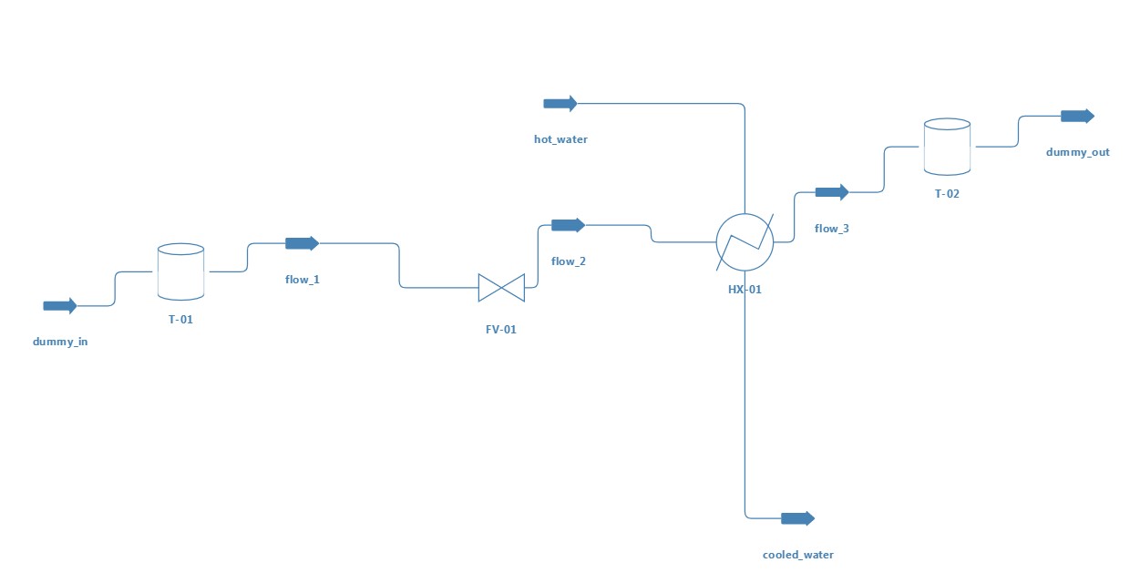
Our process consists of a heat exchanger which cools a hot water stream using cold water, stored in a tank. A valve controls the cold water flow from the source to the sink tank.

Setup

1. Create a new simulation.
2. Add Water as the single compound.
3. Add an instance of the IAPWS-IF97 Property Package.

Build

1. Add, name and connect the flowsheet objects as per the above screenshot.
2. Set the dummy_in mass flow to 23.6155 kg/s.
3. Set the hot_water mass flow to 7.46 kg/s.
4. Set the hot_water temperature to 397 K.
5. Set the hot_water pressure to 1000000 Pa.
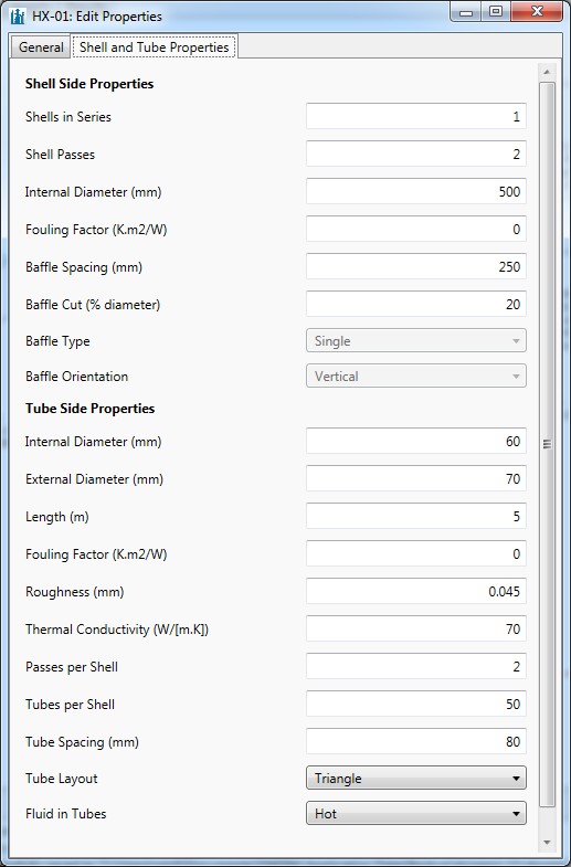
6. Set the heat exchanger (HX-01) calculation mode to "Shell and Tube (Rating)", with the following geometry:

Run

Press F5 to run the model. After running the model, the hot water outlet temperature should be about 323.15 K (50 C), which is our primary objective - to control the outlet temperature of the hot water stream always near 50 C.

What happens if the hot water flow rate changes? If the flow increases, the valve should allow more cold water pass through it to compensate the increase of the hot water flow rate and keep its outlet temperature at 50 C, the opposite also being true. This would decrease the water level in the source tank and increase the level in the sink tank.

None of what was described in the above sentence is possible to simulate in a Steady-State model. In the next part of this tutorial, we will add new properties to objects and create scripts to enhance our model, making it dynamic and able to predict the overall system response when the hot water flow rate changes.

Download File

Download the simulation file with what has been done so far: dynamic_part1.dwxmz

Proceed to Dynamic Simulation Tutorial with DWSIM and Python, Part 2: Building the Dynamic Model